When the Axioma Global Multi-Asset Class Risk Model (AXGMM) is combined with the industry-leading Axioma Portfolio OptimizerTM (APO), the ability to track, tilt and hedge multi-asset class portfolios is exceptional. But its prowess in handling fixed income portfolios on their own should not be overlooked. Powered by robust, parsimonious factor models for both credit spreads and MBS spreads, along with rigorous modeling of rates, volatilities and full asset class coverage, the fixed income components of AXGMM provide an excellent risk factor basis, including specific risk, that allow APO’s portfolio construction capabilities to stand out.
Risk assessment for Portfolio I – current holdings
To illustrate the capabilities of the multi-factor fixed income risk model, we analyze the active risk decomposition of a portfolio benchmarked to a diversified US dollar fixed income portfolio consisting of around 3000 bonds, with market weights distributed as 46.2% government debt (43.5% US Treasuries and 2.7% USD foreign sovereign, quasi-sovereign and agency debt), 29.8% agency MBS pools, 22.9% corporate bonds (financial, industrial and utilities) and 1.1% supranational bonds. The benchmark yield is 123 bps with a duration of 6.44 years. The analysis highlights the sources of tracking error of the initial portfolio (Portfolio I) relative to the benchmark. In the next section we formulate constraints for APO to adjust the active risk profile while controlling turnover to show how these models can support investment decisions in construction of a rebalanced portfolio (Portfolio II).
The predictive tracking error, defined as the annualized predicted standard deviation of the portfolio return minus the benchmark return, is computed based on the covariance matrix of the fixed income risk model factor returns and the portfolio constituents’ factor exposures. We use the risk model to control the factor risk deviations from the benchmark across the major risk types of rates, credit spread, MBS spread and volatility. We also keep the portfolio weights relatively close to the benchmark weights. However, we allow the portfolio wide latitude in use of the risk budget across the risk factors and how rate risk is distributed across the asset classes. Within this freedom, portfolios can be constructed to express views on the evolution of the treasury curve term structure, credit spread or mortgage spreads.
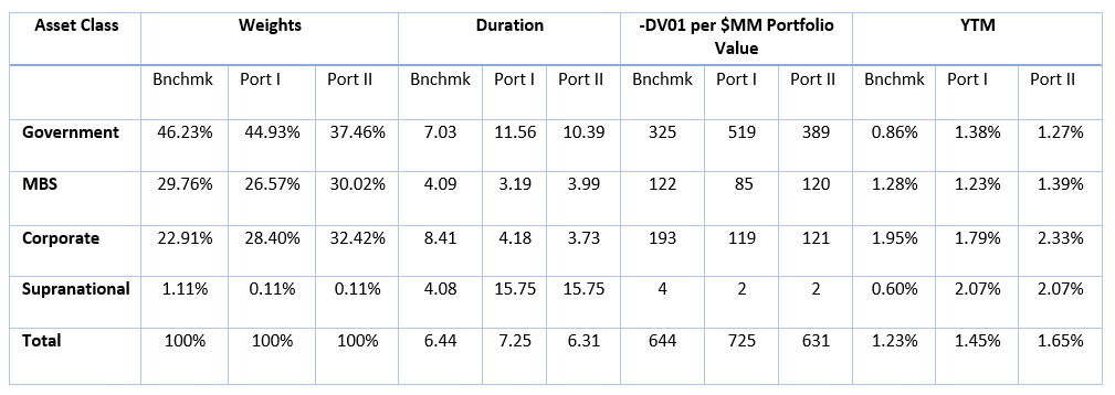
Portfolio I consists of 47 bonds with a yield-to-maturity of 145 bps, 22 bps higher than the benchmark, but a duration of 7.25 years. Portfolio I is somewhat overweight in corporate credit and underweight in government bonds and MBS relative to the benchmark. A summary of the weights, duration and yield properties by asset class of the benchmark, Portfolio I and Portfolio II can be found in Table 1. Portfolio I is consistent with a view of a flattening treasury curve, based on the significant higher government bond duration than the benchmark, balanced by shorter duration corporate bonds. However, the overall portfolio duration is still substantially higher than the benchmark.
Table 1: Effective duration and yield characteristics of Portfolios I and II and the benchmark

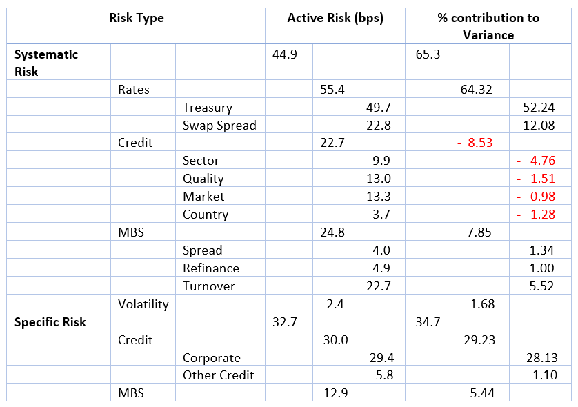
The total tracking error of Portfolio I to the benchmark is 55.5 bps. The active risk decomposition, which breaks down the sources of portfolio tracking error, is given in Table 2. For various risk types we give the absolute level of active risk in basis points as well as the percentage contribution to variance, which at each level of the decomposition is additive to the next level. At the top level, the percentage contribution to variance of the systematic risk plus the percentage contribution to variance of the specific risk sums to 100%. As systematic risk and specific risk are by construction uncorrelated, this corresponds to (44.9 bps)2 + (32.7 bps)2 = (55.5 bps)2.
Table 2: Risk decomposition of total tracking error of 55.5 bps for Portfolio I relative to the benchmark

The risk decomposition shows that much of the specific risk comes from the corporate exposure, while the systematic corporate risk acts as a diversifier in the variance contribution. Treasury risk has the largest contribution to systematic variance, driven by the large difference in effective duration of the portfolio and benchmark. Within the MBS systematic risk, there is a somewhat of a tilt toward Turnover risk.
Rebalancing into Portfolio II
Suppose we would like to tighten the tracking error to the benchmark a bit and substantially increase the yield of the portfolio. We observe from the risk decomposition that much of the active variance is coming from rates corresponding to the duration mismatch, while little is coming from systematic corporate spread risk. Therefore we would like to shift the risk budget from rates to credit. If we somewhat reduce the exposure to long maturity treasuries and shift to higher yielding corporates, it is likely that we can achieve a significant increase in yield. In APO, this can be achieved capping the portfolio weight of individual bonds at 5% and tightening up the constraints for matching key rate durations. As a practical matter, it is also important to minimize the turnover required to achieve these goals.
We therefore set up the following rebalancing in APO. Starting from the original portfolio, we seek to minimize turnover (total dollar amount traded) subject to several constraints. These include requiring the portfolio yield-to-maturity to be at least 40 bp larger than the benchmark while capping the difference between the portfolio and benchmark key rate durations at +/- 0.01 years to reduce rate risk. We also constrain total tracking error to be less than or equal to 50 bps, as well as limit the systematic MBS and Volatility active risk to 10 bps each. To control transaction costs, holdings and trades are required to be at least 0.05% of the portfolio. A cap of 5% weight on any individual bond is also imposed.
Portfolio II has 45 bonds and a yield-to-maturity of 165 bps, representing a 42 bps increase in yield over the benchmark. The new duration is 6.31 years, corresponding to a substantial decrease in rates active risk. This requires selling off all of 16 bonds and part of the position in 10 bonds in the original portfolio, corresponding to 32.36%, and buying 14 new bonds. Table 1 shows the weights, durations and yields for the Portfolio II.
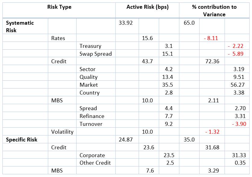
The total tracking error to the benchmark is now 44.1 bps. Table 3 shows the active risk decomposition of Portfolio II. As expected, we see the contribution of rates to active variance is much smaller, while credit now accounts for 104% of variance, with systematic credit at 72.4% and specific credit at 31.7%. MBS risk has decreased somewhat, now accounting for only 2% of active variance.
Table 3: Risk decomposition of total tracking error of 44.1 bps for Portfolio II relative to the benchmark

Conclusion
This example shows how the risk analysis of AXGMM can be paired with the portfolio construction capabilities of APO to achieve investment goals. Of course there are many other directions to explore in rebalancing. These may include tightly controlling turnover, incorporating a liquidity constraint on the names traded, or seeking to hedge out the some of the active credit market risk. The flexibility of APO and the power of the AXGMM risk model deliver the tools that allow portfolio managers to act on their insight when building fixed income portfolios.


